Dose Finding

Determining the optimal dosage is a crucial aspect of a clinical trial. Administering less than the optimal dose may not effectively treat the patient while giving more than that could lead to irreversible side effects. Therefore, finding the optimal dosage during the first two phases is one of the primary objectives. The methods used in determining the best dose for each phase differ due to the distinct goals and conditions of each phase. In the first phase, The researcher needs to determine the Maximum Tolerated Dose(MTD) and in the second phase needs to determine the Minimum Effective Dose (MED). Over time, various researchers have introduced different methods to discover them. The following diagram shows a summary of dose finding methods in clinical trials.

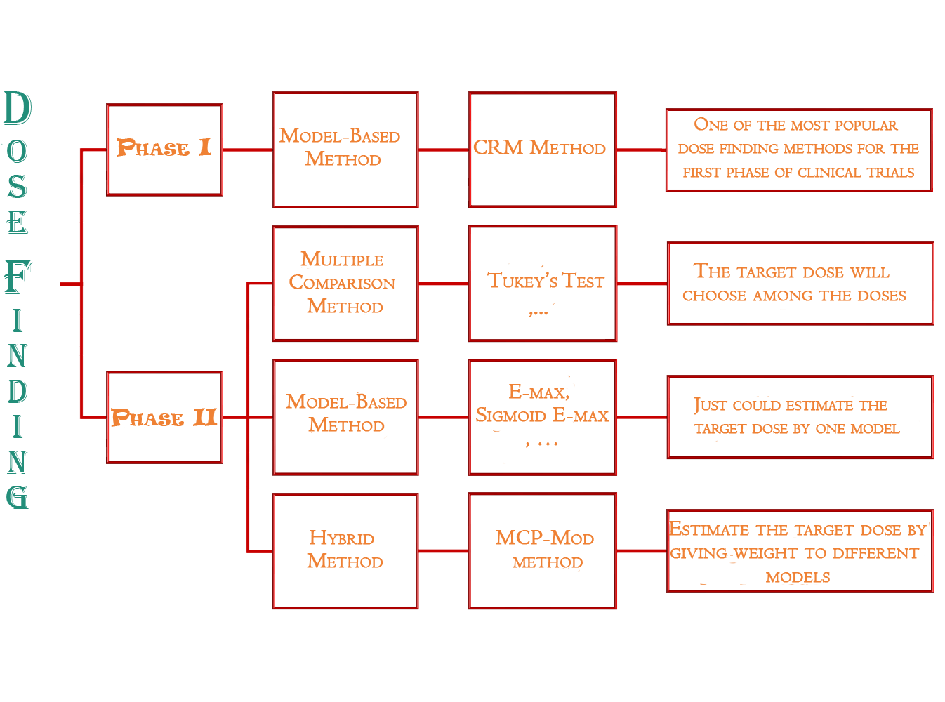
Dose Finding in the First Phase of a Clinical Trial

Here, we focus on the Continued Reassessment Method (CRM) (Wheeler et al. 2019), a widely used approach for determining the Maximum Tolerated Dose (MTD) during the initial phase of clinical trials.

How the CRM algorithm works

Applying the code to the data could provide us with a more comprehensive understanding of this approach. At first, we need to install and load the CRM package in R.

Code

# install.packages("CRM")  # remove '#' for the first time to install the package
library("CRM")

To proceed to the next stage, the researcher needs to first identify the maximum dosage that causes a tolerable level of side effects, such as 0.2 or 20%. This is known as the Target Level of Toxicity. If the toxicity level goes beyond 0.2, the researcher must reduce the dose for the next patient. Additionally, the researcher should determine the initial doses and prior toxicities, which are typically determined in the lab. For example, the prior toxicities could be 0.05, 0.1, 0.2, 0.3, 0.5, and 0.7, corresponding to dose levels 1, 2, 3, 4, 5, and 6, respectively.

Code

target <- 0.2
prior <- c(0.05,0.1,0.2,0.3,0.5,0.7)

To start the trial, administer a specific dose level to the first patient. If there are no signs of toxicity, increase the dosage for the next patient. But if there are any signs of toxicity, reduce the dosage for the following patient. For example, suppose the researcher gave dose level 3 to the first patient and did not observe any adverse reactions.

Code

# patient 1 -----------------------------------------------------
dose <- c(3)
toxicity <- c(0)

Note: The toxicity vector in the above code indicates weather each patient experienced toxicity (side effect) (1) or not (0).
After creating a matrix by combining dose and toxicity vectors, we can use crm function to find the proposed dose for the next patient.

Code

# create a matrix to store patients data
ptdata <- cbind(dose, toxicity)
res <- crm(target, prior, ptdata)
res$MTD

[1] 4

As we see, the method proposed dose level 4 for the next patient. So, if we don’t see any toxicity for this patient, the crm suggestion for the third patient would be as follow:

Code

# patient 2 -----------------------------------------------------
dose <- c(3,4)
toxicity <- c(0,0)
ptdata <- cbind(dose, toxicity)
res <- crm(target, prior, ptdata)
res$MTD

[1] 4

We repeat this process until all patients receive one of the doses of the medication.

Code

dose <- c(3,4,4,3,3,2,1,1,1,2,2,2,2,2,2,2,2,2,2,2,2,2,2,2,1)
toxicity <- c(0,0,1,0,1,1,0,0,0,0,0,0,1,0,0,0,0,0,1,0,0,1,0,1,1)
ptdata <- cbind(dose, toxicity)
res <- crm(target, prior, ptdata)
res$MTD

[1] 1

The last result shows the Maximum Tolerated Dose (MTD).

Dose Finding in the Second Phase of a Clinical Trial

Various methods have been proposed to determine the Minimum Effective Dose (MED).

1. Multiple comparison methods (ANOVA’s Post-Hoc):

Dunnett’s Test
Bonferroni Correction
Tukey’s Test
…

The constraint of the multiple comparison methods: The target dose would be among the doses which the researcher determined them and we couldn’t assess any doses in the range of them.

The solution: The modeling methods are presented.

2. Modeling methods:

The Sigmoid Emax Model
The Logistic Model
The Quadratic Model
…

The constraint of the modeling methods: We just use one model for finding the target dose which may not be the best model for finding the target dose.

The solution: using hybrid methods like MCP-Mod

3. Hybrid methods:

MCP-Mod (Multiple Comparison & Modeling)(Bornkamp, Pinheiro, and Bretz 2009)

A two steps approach:
MCP step: This step is designed to identify a dose-response signal (i.e., the dose-response curve shouldn’t be flat) applying multiple comparison procedures.
- It helps to confirm that the drug works as intended there is a measurable response that changes with the dose
❌ If this step fails to establish a dose-response signal, it may indicate that the drug doesn’t have the desired effect, or the effect doesn’t vary with the dose.
✅ Once the MCP step has established a dose-response signal, the process moves on to the Mod step, which estimates the dose-response curve and the target doses of interest using modeling techniques
Mod step: This step estimates the dose-response curve and target doses of interest (such as ED 50, ED 90, MED, etc.) with combining multiple modeling techniques.

Code

# install.packages("DoseFinding")
library("DoseFinding")
library(ggplot2)
library(sjPlot)
data(biom)
models <- Mods(linear = NULL, linlog = NULL, emax = 0.2, exponential = 0.7, doses = c(0,0.05,0.2,0.6,1))
## perform MCPMod procedure
mm_aic <- MCPMod(dose, resp, biom, models, Delta = 0.4, alpha = 0.05, selModel = "aveAIC")
## evaluate MCP-Mod

# summary(mm_aic)   # do uncomment if you want to see the results 

plot(mm_aic, plotData="meansCI", CI=TRUE)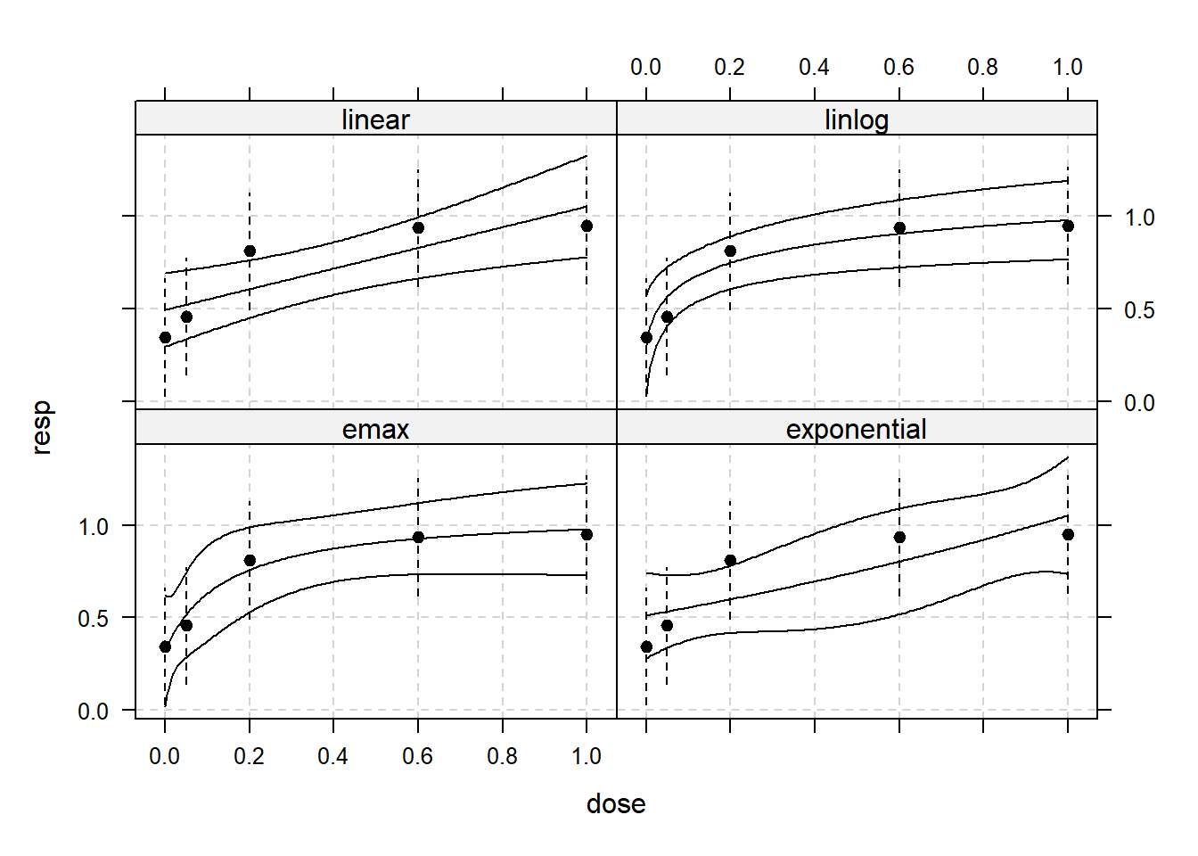

Based on the graph, it appears that the “linlog” and “emax” models have performed better. These models have curves that closely match the observed data points, and none of the data points lie outside the confidence band when compared to the other models.

Code

modweights <- mm_aic$selMod

## model avaraged dose-estimate
TDEst <- mm_aic$doseEst %*% modweights
TDEst

          [,1]
[1,] 0.2497399

The Minimum Effective Dose (MED) is the weighted average of significant model results.

References

Bornkamp, Björn, José Pinheiro, and Frank Bretz. 2009. “MCPMod: AnRPackage for the Design and Analysis of Dose-Finding Studies.” Journal of Statistical Software 29 (7). https://doi.org/10.18637/jss.v029.i07.

Wheeler, Graham M., Adrian P. Mander, Alun Bedding, Kristian Brock, Victoria Cornelius, Andrew P. Grieve, Thomas Jaki, et al. 2019. “How to Design a Dose-Finding Study Using the Continual Reassessment Method.” BMC Medical Research Methodology 19 (1). https://doi.org/10.1186/s12874-018-0638-z.